This is PART II of series of SVM.
Link is here for PART I of SVM
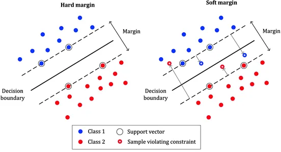
In the last story we learn to find an optimal hyperplane from the set of hyperplane which separate the two classes and stays as far as from closest data-points (support vector). No data points are allowed in the margin areas. This type of linear classification is known as Hard margin classification.
But here is the problem with hard margin classification!!

If we strictly impose that hyperplane stays as far as from the closest data points,then the data points will be linearly separable but there will be also narrow margin, in that case model will be extremely sensitive to noisy data points , and model will lack generalization capability i.e. chance of under-fitting will increases. Also, it will only work with linearly separable data-points(training example). data points and training example are interchangeable words referring to same thing.
so what should we do??
To avoid these issues it is preferable to use more flexible model. As most of real world data are not fully linearly separable, we will allow some margin violation to occur. It is better to have large margin, even though some constraints is violated. Margin violation means choosing an hyperplane, which can allow some data points to stay in either in between the margin area or in the incorrect side of hyperplane,which is contrast to hard margin classification task . This type of classification are called as soft margin classification.
what does it mean Mathematically??
we will relax the constrains of the equation slightly to allow the margin violation to occur with the help of positive slack variable ξi. so now above equation can be written as,

ξi actually tells where the ith observation is located relative to hyperplane and margin,for 0<ξi≤1, then observation is between incorrect side of margin and correct side of hyperplane.This is margin violation. for ξi>1 ,observation is on the incorrect side of both hyperplane and margin, and point is misclassified. And in the soft margin classification task, the observation is on the incorrect side of margin have penalty which increases as distance from it increases.
C is the parameter which controls the trade-off between length of margin and number of the misclassification on the training data. For C=0, It is not letting any misclassification to occur which is a nothing but hard margin classification and it result in narrow margin, For C>0, it mean no more than C observation can violate the margin, as C increases margin also widens.
The correct value of C is decided by cross-validation and it is this parameter only, that can result in bias-variance trade-off in SVM. If the value of C =0, which results in high variance but if the value of C= ∞ it results in high bias.
Optimization
As we seen in last part of SVM, the learning problem of Hard margin classifier is formulated as Dual quadratic Programming Problem. we have also understand the concept of primal and dual optimization problem.
The soft margin optimization will be similar to that hard margin optimization task, but it will include an additional penalty term which penalize margin when a data point is mis-classified. The loss function is given as,

If you remember Primal optimization problem, then you can see that above equation is also Primal optimization problem
Learning SVM Soft Margin classification can also be formulated in two ways;
- Primal gradient based optimization method
- Dual quadratic programming based method
Primal gradient based optimization method
This is most popular optimization algorithm for SVM’s soft margin classification task. As we already discussed in PART I, that SVM optimization problem is a constrained optimization problem which can not be solved with the gradient descent optimization algorithm. But if we somehow make optimization problem into an unconstrained form -without Lagrange multipliers, that can be directly compared to other kinds of linear classification, then in that case we can use gradient decent to update the parameters of classifier.
can we do this??
yes!!!! lets see below series of steps,

If you look the loss function, you can see clearly that it compose of two term,first is regularizer term and second is loss function term. The loss function term in below is Hinge loss.

So, Cost function c(w,b) for l numbers of training examples can be written as,

where λ =2/(LC) and f(x)= w.x+b
We got the loss function, and then using gradient descent algorithm, we can update the parameters.
Dual quadratic programming based method
It will be similar to Hard margin classification task, so i will not explain and derive the equation in details, there will be only change in upper bound of λ in the loss function, which is now C. So, optimization algorithm can be written as,

Now which of above optimization is good???
The dual quadratic programming method converge easily as compared to Primal gradient based method, but the quadratic based method is not scalable in case of large data-set and also in case of online learning, dual problem fails. In contrast gradient based approach work very well on large data set and online learning is also possible. Also, kernel trick which we cover in 3rd tutorial is only possible with dual optimization.
so both are good depending on our problem statement
Thank you for reading. In next story we will cover the case when data point is non-linear separable.