This is PART III of SVM Series

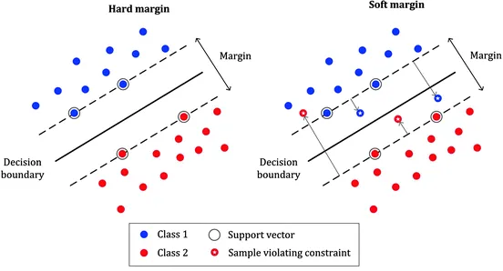
Last two part on SVM, we talk about the data points are either partially or fully linearly separable, knows as soft and hard margin classification task respectively.
What if data points is not at all linearly separable ?, What if data points are scattered in shape of circle?
So we need a generalized version of SVM which can perform well on any type of data shape, it doesn’t care if your data points have linear shape, circular, ellipsoid or any thing, it just care about finding an optimal decision boundary that divides both the two class .
Before diving deeper into concept, lets discuss few mathematical theorem and relation which are very crucial to understand this whole story.
Mercer’s Theorem:
It says if a function K(a,b) satisfy all the constrains called mercer’s constrains, then there exists a function that maps a and b into higher dimension.

So, in this story we will talk about formulation of SVM which can deal with any shape of data points.
So how we will do that??
kernel trick!!!!!
what the heck is this kernel trick now??
It is method of using linear classifier to classify non-linear data points. Mathematically, it is above explained Mercer’s theorem, which maps non-linear input data points into higher dimension where they can be linearly separable. And kernel is a function which actually perform the above task for us. There are different types of kernel like ‘linear’, ‘polynomial’, ‘redial basis function’ etc. Selecting a right kernel which can best suit your data is obtained by cross-validation.
Small visualization of how ‘polynomial’ kernel can separates non-linear data into linearly separable in higher dimension. From the below figure you can see 2D plane data is linearly separated in 3D plane.

So how do you actually use this kernel trick ??
In the PART I of SVM, Dual optimization problem is broken down to below maximization problem,


So solving the above minimization problem. you will get the value of λ, then using it, we will compute w and b. The λ dependent equation of w can be seen in PART I of the SVM. And from w we will compute b.
As we now have the value for both w and b , then optimal hyperplane that can separates the data points can be written as,
w.x + b = 0
And a new example x_ can be classified as sign(w.x_ +b)
But till now everything is fine, but did you guys feel something in mind like, instead of using kernel trick at time of optimization why can’t we transform out input data points into higher dimension and then use soft-margin classification to predict the classes??? can we do this??
yes we can do something like that, but here is a catch, if you transform whole input data into higher dimension data then you guys need lots of space and computational cost will increase many fold as compared to kernel trick. so that’s why we use kernel trick during optimization process.
Popular kernel
Gaussian Redial basis function
It is one of the most popular kernel used in SVM. It is used when there is no prior knowledge about data.

Gaussian function
It is written as,

Polynomial Kernel Function
It is written as,

Linear Kernel
It is just the normal dot product,

Small comparison of all the above kernel,

It is always recommended to use as simple model as you can, only go for complex model like kernel trick if required.
That’s it about Kernel Trick and SVM. Thanks for reading. Hope you have understand the concept of SVM well. If you have any doubt you can comment and ask!!!